Page Comparison

Once the data preparation step is finished, we can continue with the development of the AI algorithm. As seen earlier, the data preparation supposes the data cleaning (managing null errors or missing values or errors), field/feature selection, conversion of categorical data, normalization and randomization of ordering. Each AI algorithm may demand a specific data preparation, at least in terms or normalization and randomization of ordering.

Data segregation

The AI model training and evaluation includes the data segregation, the model training and evaluation. The data segmentation corresponds to the splitting the database into of the data in two (train and test sets) or three data sets (train, development and test sets) depending of the validation procedure that was selected.

Generally, the splitting of the dataset into training and test sets (and sometimes training/development/test sets) through a simple process of random subsampling. However, as we deal with skewed datasets , it is important to verify that the subsampling does not alters the statistics - in terms of mean, proportion and variance - of the sample. Indeed, the test set may contain only a small proportion of the minority class (or no instance/entity at all). In order to avoid this, a recommended practice is to divided the dataset in a stratified fashion, i.e. we randomly split the dataset in order to assure that each class is correctly represented (we will thus maintain in the subsets the same proportion of classes as the complete dataset). Common training/test ratios are 60/40, 70/30, 80/20 or 90/10 (for large datasets).

The training dataset is the data we are using to train the model, i.e. to estimate the parameters and hyperparameters describing the models. The test set allows the evaluation of the estimated model parameters and hyperparameters.

The development dataset (known also as validation set) allows an unbiased evaluation of the model fit on the training dataset, while estimating the model hyperparameters. This set is only used to fine-tune the hyperparameters of the model, but not the model parameters and thus will only indirectly affect the model.

The test set allows the evolution of the estimated model parameters and hyperparameters.

The train/dev/test split ratio is specific to each use case, the number of samples and the model that we are trying to train. This methodology for splitting the data allows to detect bias and variance problems.

As one (item/service) observation in the database depend on several variables, we are dealing with multi-variable anomaly detection problems. As seen earlier, several machine learning algorithms can meet the proposed goals of this project. As the data is partially labeled, unsupervised learning techniques like Robust Covariance, One-Class SVM and Isolation Forest usually give satisfactory results. These techniques are based on the principle of identifying groups of similar data points (and implicitly corresponding to the normal class, i.e accepted items and services) and considering the points exterior to these groups as anomalies/abnormal observations (rejected items or services).

For the Robust Covariance technique, the basic hypothesis is that the normal class have a Gaussian distribution. The train set- composed only of normal class observations – will allow the estimation of the parameters of the Robust Covariance model: the mean and covariance of the multivariate Gaussian distribution. The threshold of the model able to separate the normal and abnormal classes is further estimated based on the development set and taking into account the trained parameters of the model. The test set will allow to evaluate the performance of the trained algorithm. A possible splitting of the data for this algorithm can be:

• training set composed of 60% of the normal data;

• development set composed of 20% of normal data and 50% of the abnormal observations;

• test set composed of the remaining 20% of normal observations and 50% of abnormal ones.

One-Class SVM algorithm relaxes the hypothesis that all the fields/columns in the normal class must have a Gaussian distribution. Thus, it identifies arbitrary shape regions with a high density of normal points and classify as anomaly/outlier any point that lies outside the boundary. Here again the algorithm is trained only on part of the normal class.

Isolation Forests are constructing a collection of decision trees, in which each decision tree splits the data along a random point and without considering any hypothesis on the shape of the distribution. Anomalies are considered as being the most isolated points. In this case the training set must contain normal class and abnormal class observations.

AI model training and evaluation

The AI models documented here correspond to AI models that have obtained at least an f1-score of 0.60 on the evaluation step. All the selected models are part of the classification based Anomaly detection techniques and correspond to Decision Trees, Random Forest, Extra-Trees, Extra Gradient Boost and Voting Classifier.

AI model dependencies

For the present case, we have used the following dependencies:

• Feature engineering: two feature configurations were tested (1) Features1: 27 selected features after the data analysis and visualization; (2) Features2: the previous 27 selected features and 6 aggregated features (related to submitted items and related amount by the insurer per week, month, year)

• Rejected entities for missing document(s) or modified according to document(s) were not consider in the study (as there is no feature related to the submitted/necessary documents)

• Normalization method: (0) no normalization; (1) Mean and standard deviation normalization; (2) Median and IQR normalization; (3) Minimum and maximum normalization

• Data segregation: training set composed of 90% of all labeled data; test set composed of 10% of the labeled data set

• Hyperparameter tunning: we have used a stratified k-fold cross validation procedure, which allows us to have the same data distribution of data for training and validation while having an accurate validation scheme for testing different hyperparameters configurations.

Decision Tree Classifier

The hyperparameters tuned for the Decision tree Classifier are:

• criterion: measuring the impurity of the split with possible values: ‘gini’ (default value) and ‘entropy’

• maximum depth of the tree, with values from 5 to 61 (default is ‘None’)

• minimum number of entities contained in a node in order to consider splitting with possible values between 4 and 40 (default value is 2)

• minimum number of entities contained in a leaf with possible, with possible values between 3 and 40 (default value is 1)

The confusion matrix obtained for the Decision Tree Classifier with the default values is the following

...

Based on the confusion matrix, we can compute the evaluation metrics considered in this study:

• Precision = 0.6794 (i.e. from all entities predicted as rejected, 67.94% were correctly classified)

• Recall =  0.6023 (i.e. from all entities rejected by the Medical Officers, the classifier correctly categorized 60.23%)

• f1 score = 0.6385

• Accuracy = 0.9819 (I.e. from all the entities considered, 98.19% of items were correctly categorized)

 In terms of  execution time, the training time was about 80.94 s, while the prediction time was 0.08 s on the computed configuration mentioned earlier.

The default parameter values for the Decision Tree Classifier are the following: criterion = ‘gini’, splitter = ‘best’, max_depth = None, min_samples_split = 2, min_samples_leaf = 1, min_weight_fraction_leaf = 0, max_features = None, random_state = None, max_leaf_nodes = None, min_impurity_decrease = 0, min_impurity_split =0, class_weight = None, ccp_alpha = 0.

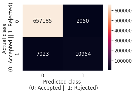
The best hyperparameters obtained correspond to criterion = ‘entropy’, max_depth = 20; min_samples_leaf = 20, min_samples_split = 22 (for the other parameters, the default values were considered). The confusion matrix, evaluation time and evaluation metrics are given below. While the False Negative cases have slightly increased with respect to the previous prediction, the False Positive entities have decreased from 5'109 to 2’920 (and implicitly a higher Precision value)

...

Evaluation metrics on the test set:  Precision = 0.7864; Recall = 0.5980; f1-score = 0.6794; Accuracy = 0.9850

 The training set was composed of 677’212 entities, with 659’235 accepted and 17’977 rejected entities.

Random Forest

The confusion matrices obtained with the Random Forest Classifier, for the test dataset, with the default parameter values is the following:

...

Based on the confusion matrix, we can compute the evaluation metrics considered in this study: Precision = 0.8112; Recall = 0.6134; f1-score = 0.6986; Accuracy = 0.9859

The default parameter values for the Random Forest Classifier are: n_estimators = 100,  criterion = 'gini',  max_depth = None,  min_samples_split = 2, min_samples_leaf = 1, min_weight_fraction_leaf = 0.0, max_features = 'auto', max_leaf_nodes = None, min_impurity_decrease = 0.0, min_impurity_split = None, bootstrap = True, oob_score = False, n_jobs = None, random_state = None, verbose = 0, warm_start = False, class_weight = None, ccp_alpha = 0.0, max_samples = None.

The hyperparameters tuned for the Extra-Trees Classifier are:

• criterion:  “gini” and “entropy”

• maximum depth of the tree, with values from 5 to 81

• maximum features: ‘auto’ (random subset of features considered), ‘sqrt’, ‘log2’, ‘None’ (all features are considered)

• minimum number of entities contained in a node in order to consider splitting with possible values between 4 and 40 (default value is 2)

• minimum number of entities contained in a leaf with possible, with possible values between 4 and 40 (default value is 1)

• bootstrap: [False, True]

• Class_weight: [‘balanced’, None]

• n_estimators: [10, 50, 100]

The best parameters obtained are the following: n_estimators = 100; min_samples_split = 4; min_samples_leaf = 6; max_features = ‘sqrt’, max_depth = 25; criterion = entropy; class_weight = None, bootstrap = False and having the giving the confusion matrices and evaluation metrics: Precision = 0.8424; Recall = 0.6093; f1-score = 0.7071; Accuracy = 0.9866

Image Added

Extra-Trees Classifier

The evaluation metrics obtained by the ExtraTrees Classifier with the default parameter values are the following: Precision = 0.7838; Recall = 0.6086; f1-score = 0.6852; Accuracy = 0.9852, while the confusion matrix is illustrated in the following figure:

...

The default parameter values for this classifier are: criterion='gini', n_estimators = 100, max_depth = None,  min_samples_split = 2,  min_samples_leaf = 1,  min_weight_fraction_leaf = 0.0,  max_features = 'auto',  max_leaf_nodes = None,  min_impurity_decrease = 0.0, min_impurity_split = None, bootstrap = False, oob_score = False, class_weight = None, ccp_alpha = 0.0, max_samples = None.

 The hyperparameters tuned for the Extra-Trees Classifier are:

• criterion:  “gini” (default value) and “entropy”

• maximum depth of the tree, with values from 5 to 81

• maximum features: ‘auto’ (random subset of features considered), ‘sqrt’, ‘log2’, ‘None’ (all features are considered)

• minimum number of entities contained in a node in order to consider splitting with possible values between 4 and 40 (default value is 2)

• minimum number of entities contained in a leaf with possible, with possible values between 4 and 40 (default value is 1)

• bootstrap: [False, True]

• Class_weight: [‘balanced’, None]

• n_estimators: [10, 50, 100]

 The best parameters obtained are the following: n_estimators = 100; min_samples_split = 14; min_samples_leaf = 4; max_features = None, max_depth = 75; criterion = entropy; class_weight = None, bootstrap = False and having following evaluation metrics: Precision = 0.8247; Recall = 0.6100; f1-score = 0.7013; Accuracy = 0.9862, with the confusion matrix illustrated below:

...

Extreme Gradient Boosting

Gradient Boosting represents a class of ensemble machine learning algorithms designed for classification or regression problems. These ensemble are mainly constructed from decision tree models. Trees are added to the ensemble one at a time, in order to correct the prediction error made by the previous added trees (and it is the principle used in ‘boosting’). The convergence of the models is realised using differentiable loss function and gradient descent optimization.

 Hyperparameters to be tunned:

• number of trees considered for the XGBoost ensemble (default value is 100)

• the depth of the trees added to the ensemble (default value is 6); it corresponds to the ‘max_depth’ parameter

• learning rate (default value is 0.3); it correspond to the ‘learning_rate’ parameter

• number of samples used to fit each tree (each tree can be fit on a randomly selected subset of the training set); it correspond to the ‘subsample’ parameter and can have values between 0.1 up to 1.0 (default value is 1.0); trees trained on a smaller subsample of the training dataset may show larger variance for each tree thus improving the overall performance of the ensemble

• number of features used to fit a tree or number of features used for each split, with the associated parameters ‘colsample_bytree’, respectively ‘colsample_bylevel’, with possible values between 0.1 to 1.0 (corresponding from 10% to 100% of the considered features);

• weight to consider to the minority class, with the associated parameter scale_pos_weight, and explored values between 1 to 100 (default value is 1).

 The best XGBoost model has the following parameters: number of trees = 100, max_depth = 25, learning_rate = 0.10, subsample = 1, colsample_bytree = 0.9, scale_pos_weight = 1.

Voting Classifier

The Voting Classifier considered here take into account four distinct classifiers: Decision Tree, Extra-Trees, Random Forest and Extra Gradient Boost.

The Voting Classifier can be used when:

• all the models in the ensemble must have similar good performance and in this case we chosen classifiers with a f1-score of at least 0.65 and accuracy of at least 0.98;

• all the classifiers considered mostly agrees.

The correlation matrix of the predictions obtained with the four considered classifiers is represented in Fig. Xx. As it can be observed, the results show at least 0.85 correlation index between classifiers results indicating that the classifiers mostly agrees on the predictions.

...

The hyperparameters to be tuned for the Voting Classifier are the following:

• classifiers to be selected for prediction: Decision Tree, Random Forest, Extre Trees, Extra Gradient Boost or a combination of of these classifiers

• type of voting: hard or soft; hard voting uses predicted class labels for the ensemble classifiers for majority rule voting, while soft voting will predict the class label based on the probabilities given by the classifiers.

• weights: in order to modify the importance given to the results of each classifier, i.e. giving more credit to most accurate classifiers.

The results obtained for the Voting Classifier are illustrated in the following table. The Voting Classifier with the best f1-score is the one which takes into account only three classifiers (Random Forest, Extra Trees, Extra Gradient Boost) and makes its predictions through a hard voting principle (considering only the labels predicted by the classifier in the ensemble). The evaluation of the classifiers is realized on the test set (composed of 659235 accepted item and 17977 rejected ones).